Imputing scales using parcels of items as auxiliary variables
Multiple imputation of scales generated by several items can be challenging. Fortunately, to impute every single item is not the only solution to the missing data problem. Some practical and theoretically attractive alternative have already been proposed. In this post, I show a simple implementation of what Enders (2010) calls duplicated-scale imputation, a method orginally suggested by Eekhout et al. (2011). By the way, thanks Iris Eekhout for replying my e-mails!
Procedure
For each scale, I define a number or proportion of items (let’s say p) to create parcels (i.e., average of items although not the whole scale). These parcels are, then, used as auxiliary variables to impute the original scales. There are different ways to define parcels. I implemented a solution in my R package sdazar, see the function rowscore for more details.
The function rowscore selects p items with the least missing data. For each case (row), it computes the parcels using the available information of the selected items. If only one item has information, only that one will be used. If there are more than one item with valid data, it will average all the selected items. If there are no items available in my initial selection, it picks p items from the rest of unselected items to impute the original scale. In this particular example, I create parcels using half of the items:
rowscore(data, items, p = 1/2, type = "parcel")The reason for using a proportion of the original items is to include as much information as possible, but preventing strong linear dependencies between variables. Ideally, parcels are complete (no missing values). However, in some cases all the items are missing, so parcels can still have missing records (although less than the original scales).
Why not just to use the average of the available items? That solution would implicitly assume that items perfectly correlate with the scale. We know that’s not a good assumption. That is why we worry about creating scales in the first place, right? Using parcels takes advantage of the available information (items with complete information) and the relationship between a portion of items and the scale.
Here I show a simple example using the National Longitudinal Study of Adolescent to Adult Health (Add Health). First, let’s look some descriptives of the variables included in the imputation. I am using information from Wave 1 and 2. The scales/scores I am imputing are depression (19 items) and GPA (4 items). Variables ending with .p are parcels with 1/2 of the items of the original scale.
dim(dats)## [1] 12976 14str(dats[, nvars, with = FALSE])## Classes 'data.table' and 'data.frame': 12976 obs. of 14 variables:
## $ female : Factor w/ 2 levels "0","1": 1 1 1 2 1 1 1 1 1 1 ...
## $ age : int 16 16 14 13 14 17 14 17 17 14 ...
## $ race : Factor w/ 5 levels "white","black",..: 2 1 1 1 2 1 3 3 3 2 ...
## $ publicass: Factor w/ 2 levels "0","1": 1 1 1 1 1 1 1 1 1 NA ...
## $ bmi : num 27.4 16.3 22.2 18.2 21.9 ...
## $ gpa1 : num 2 3.25 3.75 3.25 2.25 1 NA 2.25 NA 2.5 ...
## $ gpa2 : num 2.5 2.5 4 3.75 1.75 1.5 NA 3 1 4 ...
## $ gpa1.p : num 2.5 3.5 3.5 3 2.5 1 3.5 3 1 3.5 ...
## $ gpa2.p : num 2.5 2.5 4 3.5 1.5 2 1.5 3 1 4 ...
## $ dep1.p : num 0.2 0.7 0 0.3 0.4 0.4 0.1 1 0.6 1.2 ...
## $ dep1 : num 0.263 0.789 0 0.211 0.474 ...
## $ dep2.p : num 0.6 0.6 0.1 0.3 0.4 0.6 0.2 1.1 0.8 0.5 ...
## $ dep2 : num 0.6316 0.5263 0.0526 0.1579 0.3684 ...
## $ ppvt : int 101 75 121 96 79 97 103 89 82 120 ...
## - attr(*, ".internal.selfref")=<externalptr># create summary table using package tables
missing <- function (x) {sum(is.na(x))}
tabular(
( dep2 + dep2.p + dep1 + dep1.p + gpa2 + gpa2.p +
gpa1 + gpa1.p + age + bmi + ppvt )
~ (Format(digit = 2) * ( Heading("Mean")
* sdazar::Mean + Heading("SD")
* sdazar::Sd + Heading("Min")
* sdazar::Min + Heading("Max")
* sdazar::Max + (Heading("Missing") * missing ))),
data = dats)##
## Mean SD Min Max Missing
## dep2 0.58 0.39 0.00 2.95 68.00
## dep2.p 0.58 0.43 0.00 3.00 6.00
## dep1 0.58 0.39 0.00 2.84 81.00
## dep1.p 0.62 0.44 0.00 3.00 18.00
## gpa2 2.86 0.74 1.00 4.00 4710.00
## gpa2.p 2.76 0.84 1.00 4.00 1238.00
## gpa1 2.82 0.76 1.00 4.00 2788.00
## gpa1.p 2.74 0.85 1.00 4.00 342.00
## age 15.28 1.61 11.00 21.00 9.00
## bmi 22.37 4.42 11.47 63.47 353.00
## ppvt 100.17 15.00 13.00 146.00 568.00As expected, the correlation between the scales and parcels is high. GPA has most of the problems. Note that parcels .p still have missing records, although much less than the original scales.
cor(dats[, .(dep1, dep1.p)], use = "complete")## dep1 dep1.p
## dep1 1.000 0.947
## dep1.p 0.947 1.000cor(dats[, .(dep2, dep2.p)], use = "complete")## dep2 dep2.p
## dep2 1.000 0.948
## dep2.p 0.948 1.000cor(dats[, .(gpa1, gpa1.p)], use = "complete")## gpa1 gpa1.p
## gpa1 1.000 0.888
## gpa1.p 0.888 1.000cor(dats[, .(gpa2, gpa2.p)], use = "complete")## gpa2 gpa2.p
## gpa2 1.000 0.885
## gpa2.p 0.885 1.000Let’s now impute the scales/scores using the R package MICE.
ini <- mice(dats[, nvars, with = FALSE], m = 1, maxit = 0)

# get methods
(meth <- ini$meth)
## female age race publicass bmi gpa1 gpa2 gpa1.p gpa2.p dep1.p dep1 dep2.p dep2 ppvt
## "" "pmm" "" "logreg" "pmm" "pmm" "pmm" "pmm" "pmm" "pmm" "pmm" "pmm" "pmm" "pmm"# get predictor matrix
pred <- ini$predI adjust the predictor matrix to avoid feedbacks during the imputation (circularity between variables). The trick is to use only complete variables when imputing parcels.
# predict parcels only with complete variables to avoid feedbacks
pred["gpa1.p", ] <- 0
pred["gpa2.p", ] <- 0
pred["dep1.p", ] <- 0
pred["dep2.p", ] <- 0

pred["gpa1.p", c("female", "race")] <- 1
pred["gpa2.p", c("female", "race")] <- 1
pred["dep1.p", c("female", "race")] <- 1
pred["dep2.p", c("female", "race")] <- 1

# predict scales using parcels
pred[, "gpa1.p"] <- 0
pred[, "gpa2.p"] <- 0
pred[, "dep1.p"] <- 0
pred[, "dep2.p"] <- 0

pred["gpa1", c("gpa1.p")] <- 1
pred["gpa2", c("gpa2.p")] <- 1
pred["dep1", c("dep1.p")] <- 1
pred["dep2", c("dep2.p")] <- 1
Here the adjusted predictor matrix:
##           female age race publicass bmi gpa1 gpa2 gpa1.p gpa2.p dep1.p dep1 dep2.p dep2 ppvt
## female         0   0    0         0   0    0    0      0      0      0    0      0    0    0
## age            1   0    1         1   1    1    1      0      0      0    1      0    1    1
## race           0   0    0         0   0    0    0      0      0      0    0      0    0    0
## publicass      1   1    1         0   1    1    1      0      0      0    1      0    1    1
## bmi            1   1    1         1   0    1    1      0      0      0    1      0    1    1
## gpa1           1   1    1         1   1    0    1      1      0      0    1      0    1    1
## gpa2           1   1    1         1   1    1    0      0      1      0    1      0    1    1
## gpa1.p         1   0    1         0   0    0    0      0      0      0    0      0    0    0
## gpa2.p         1   0    1         0   0    0    0      0      0      0    0      0    0    0
## dep1.p         1   0    1         0   0    0    0      0      0      0    0      0    0    0
## dep1           1   1    1         1   1    1    1      0      0      1    0      0    1    1
## dep2.p         1   0    1         0   0    0    0      0      0      0    0      0    0    0
## dep2           1   1    1         1   1    1    1      0      0      0    1      1    0    1
## ppvt           1   1    1         1   1    1    1      0      0      0    1      0    1    0
Let’s impute the data!
imp <- mice(dats[, nvars, with = FALSE], pred = pred, m = 5, maxit = 10)Below some plots to explore how the imputation goes.
plot(imp, c("gpa1", "gpa2", "dep1", "dep2"))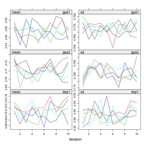
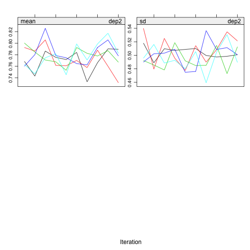
I don’t see any problematic pattern. It seems I get a proper solution. The distribution of the variables also looks right.
densityplot(imp, ~ gpa1 + gpa2 + dep1 + dep2)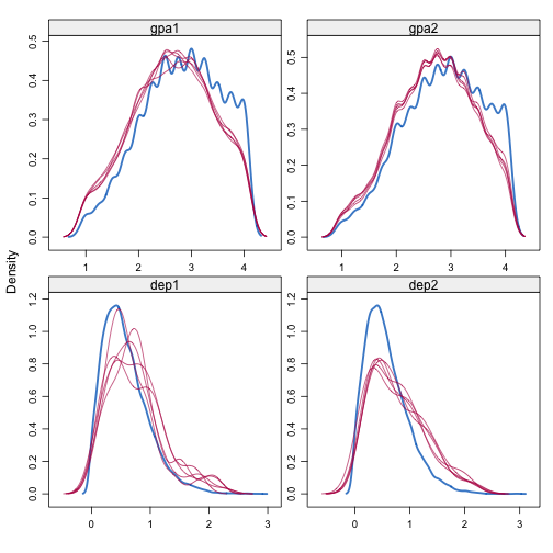
bwplot(imp, gpa1 + gpa2 + dep1 + dep2 ~ .imp)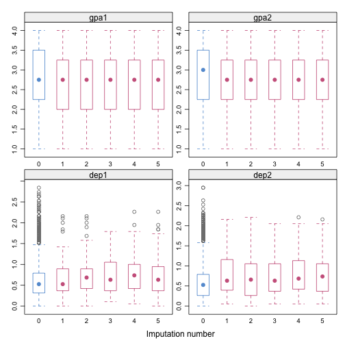
Last Update: 06/02/2017
References
Enders, Craig K. 2010. Applied Missing Data Analysis. The Guilford Press.
Eekhout, Iris, Craig K. Enders, Jos W. R. Twisk, Michiel R. de Boer, Henrica C. W. de Vet, and Martijn W. Heymans. 2015. “Analyzing Incomplete Item Scores in Longitudinal Data by Including Item Score Information as Auxiliary Variables.” Structural Equation Modeling: A Multidisciplinary Journal 22 (4):588-602.